
Content
Table of Contents
1. Requirement
There are multiple jobs running on the server, and we need to calculate precise running time metrics for each user. The system must be capable of generating reports at various time granularities: hourly, daily, weekly, and monthly. These reports are essential for resource allocation, billing, and performance analysis.
2. Technical Design
2.1 Core Data Architecture
Job running time represents historical data - once a job completes, the records exist permanently and cannot be modified. To optimize query performance, we implement a multi-tier storage strategy with separate tables for hourly, daily, weekly, and monthly aggregations.
This approach significantly reduces query latency for reports spanning longer time periods, as the data is pre-aggregated rather than calculated on demand.
2.2 Initial Job Time Sampling - Hourly Granularity
The hourly sampling serves as the foundation for our entire aggregation system. All coarser time granularities (day, week, month) are derived from this hourly data.
The core challenge is calculating the precise duration a job runs within each hour window. This requires finding the intersection between two time segments:
- The job’s lifetime (from start to end)
- The specific hour sampling window
We compute this intersection using a time-segment intersection algorithm that handles four distinct cases (explained in section 3.3).
In this diagram:
- The horizontal axis represents time
- The vertical bars delineate hour boundaries
- The colored segments represent job lifetimes
- The intersection between job lifetimes and hourly windows represents the duration we calculate and store
2.3 Time Granularity Aggregation Flow
Once we have accurate hourly data, we implement a cascading aggregation pattern for coarser time granularities:
2.3.1 Daily Aggregation
Daily data aggregates from 24 hourly records:
- Job durations are summed
- User and space statistics are averaged or counted as appropriate
- Membership snapshots are taken to track user-space relationships

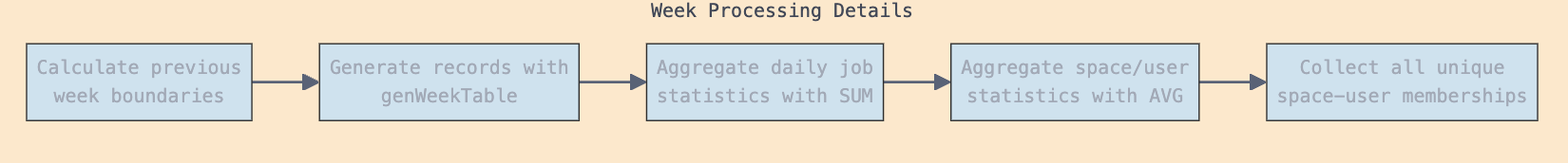
2.3.2 Weekly Aggregation
Weekly data builds upon daily records:
- Records from 7 consecutive days are combined
- Special handling for week boundaries ensures consistency
- Summary statistics calculate total resource usage per week
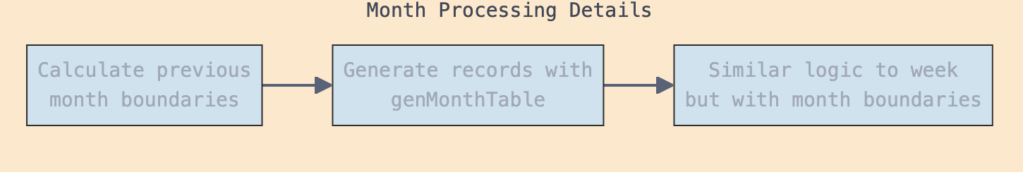
2.3.3 Monthly Aggregation
Monthly aggregation follows similar principles to weekly:
- Aggregates all daily records within the calendar month
- Accounts for varying month lengths (28-31 days)
- Provides the highest-level overview of system usage
3. Key Features and Edge Case Handling
3.1 Recursive Time Period Checking
The system implements a comprehensive backward-looking mechanism to ensure data completeness:
- Hourly: Examines past 24 hours
- Daily: Looks back 5 days
- Weekly: Checks previous 2 weeks
- Monthly: Verifies previous month
For each missing period discovered, the system creates new job status records with a jobNotExecute status, triggering subsequent processing.
Importantly, the backward search is bounded by the oldest record in the database. This prevents unnecessary processing of ancient time periods while ensuring that no recent periods are missed.
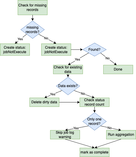
3.2 Dirty Data Handling
Data integrity is paramount. Before processing any period marked as “not executed,” the system:
- Checks if data already exists for that period in the target table
- If found, it designates this as “dirty data” (potentially incomplete or inconsistent)
- Removes this dirty data completely
- Proceeds with fresh aggregation from source data
This clean-slate approach ensures data consistency, particularly when recovering from system interruptions.
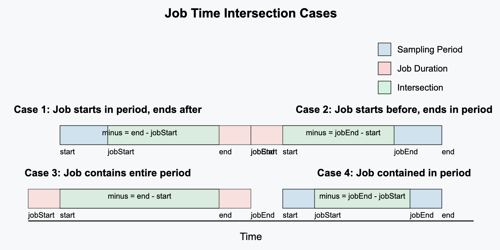
3.3 Job Duration Calculation Algorithm
The system handles four distinct cases of time intersection between jobs and sampling periods:
Case 1: Job starts within period, ends after period
- Scenario: Job begins during the sampling period but continues beyond it
- Calculation:
Duration = periodEnd - jobStart - Example: If a job starts at 10:30 AM and the sampling period is 10:00-11:00 AM, we count 30 minutes
Case 2: Job starts before period, ends within period
- Scenario: Job began before the sampling period but ends during it
- Calculation:
Duration = jobEnd - periodStart - Example: If a job started at 9:30 AM, ends at 10:15 AM, and the sampling period is 10:00-11:00 AM, we count 15 minutes
Case 3: Job spans the entire period
- Scenario: Job begins before and ends after the sampling period
- Calculation:
Duration = periodEnd - periodStart(full period) - Example: If a job runs from 9:00 AM to 12:00 PM, and the sampling period is 10:00-11:00 AM, we count 60 minutes
Case 4: Job contained entirely within period
- Scenario: Job starts and ends completely within the sampling period
- Calculation:
Duration = jobEnd - jobStart(entire job duration) - Example: If a job runs from 10:15 AM to 10:45 AM, and the sampling period is 10:00-11:00 AM, we count 30 minutes
After calculating the raw duration, the system:
- Rounds to an appropriate precision (milliseconds)
- Converts to hours (for standardized reporting)
- Multiplies by GPU count for resource-usage metrics
3.4 Deployment Protection
To handle system initialization and prevent data inconsistencies during deployment:
- The system detects if there’s only a single record in the status table
- This condition indicates first-run after deployment or system reset
- In this situation, the system intelligently skips processing that particular period
- A warning message is logged for monitoring purposes
- Normal processing resumes with subsequent periods
This approach prevents erroneous calculations during system initialization while ensuring no data gaps occur.
4. Automatic Recovery Mechanisms
To ensure resilience against system failures, maintenance windows, or other interruptions, we’ve implemented robust self-healing capabilities through a comprehensive status tracking system.
4.1 Status-Based Recovery System
Each aggregation job maintains a status record that transitions through several states:
jobNotExecute: Period identified but not yet processedjobProcessing: Aggregation in progressjobCompleted: Successfully finishedjobFailed: Encountered an error
This state machine allows the system to:
- Resume interrupted operations
- Retry failed periods
- Maintain data continuity despite interruptions
4.2 Missing Period Detection and Backfilling
The system automatically:
- Identifies time periods with missing data
- Creates appropriate status records
- Prioritizes processing based on age and importance
- Maintains chronological integrity of data
To prevent unbounded growth, the system won’t create periods before the first recorded period in the database. This establishes a natural starting point for aggregation.
4.3 Transaction Management
All database operations utilize explicit transactions with:
- Batch processing (100 records per batch)
- Automatic rollback on failure
- Detailed error logging with stack traces
- Commit verification
This approach ensures atomicity - either all operations for a period succeed, or none do, preventing partial or inconsistent data states.
4.4 Time Zone Management
Time zone consistency is critical for accurate period boundaries. The system:
- Uses explicit Asia/Shanghai time zone for all date calculations
- Ensures consistent hour/day/week/month boundaries
- Handles daylight saving time transitions properly
- Maintains accurate time alignment across all aggregation levels
4.5 Job Duration Edge Cases
The system gracefully handles several edge cases:
- Jobs with missing start times (uses default values)
- Jobs still in progress (handles null or zero EndTime)
- Zero-duration jobs (establishes minimum countable duration)
- Jobs spanning multiple periods (correctly apportions time)
- Proper rounding for partial hours (consistent decimal precision)
5. Implementation Guidelines
When implementing or extending this system, consider the following best practices:
- Data Consistency: Always maintain the aggregation hierarchy (hour → day → week → month)
- Error Handling: Log detailed information for any aggregation failures
- Performance Optimization: Index critical fields in time-series tables
- Monitoring: Implement alerts for failed aggregations or missing periods
- Scalability: Design for horizontal scaling as job volume increases
By following these guidelines and leveraging the robust recovery mechanisms, the system will maintain accurate job time metrics even under adverse conditions.